The outstanding handout by Richard Hendrickson about model trucks for freight cars, first posted on October 15 of this year, has been updated with additional information and a few corrections. It is now available on Google Drive at this link:
https://docs.google.com/file/d/0Bz_ctrHrDz4wcjJWcENpaDJYbUU/edit?usp=sharing
This was a fairly large PDF when first uploaded, but right after the first of the year (2013) we shrank it, so it should download in a reasonable time. It’s a rich source of information for any freight car modeler, and well worth any annoyance.
Tony Thompson
Saturday, December 29, 2012
Friday, December 28, 2012
Small modeling project: brass tank car
In 1988 or thereabouts, Precision Scale Company imported a slew of HO scale tank cars, with somewhat simplified construction but overall good proportions. These were apparently all “chemical” tank cars, with insulated jackets and platforms around the dome. (I think this application of the term “chemical” to all such tank cars originated with Athearn, years ago.) PSC did several car sizes, including at least 8000- and 10,000-gallon ICC 104 (non-pressure) cars, and 11,141- and 12,000-gallon ICC 105 (pressure) cars. The latter two might seem quite similar, but in fact the 12,00-gallon car was significantly longer (and slightly smaller in diameter) than the 11,141-gallon model. I know about these four because I have at least one of each:

These cars were fairly cheap and I bought a bunch, thinking that even if the paint schemes were poorly done or inaccurate, I could always repaint and re-letter them for other purposes. As it happens, the two larger-size cars did not even come with any of the smaller lettering for capacity and other specifics, typical of tank cars, and so would need additional decals even if the paint schemes were used as-is. But one of the 8000-gallon cars seemed like it could be used as it was supplied, a Celanese Chemical car.
For those who may not remember or never saw these models, here is a photo of the kind of minimal box in which they were delivered.

Examining the model out of the box, it was immediately evident that a narrow, near-scale-width coupler platform was provided, which naturally suggested use of the Kadee #78 couplers in assembled form. Sure enough, with a small amount of filing to enlarge the end-sill opening slightly, those couplers did fit all right. Here is how they looked when installed. Also note here that the car was manufactured as an all-green car, but in fact the Celanese cars had black underframes. This was corrected later.

Though not too evident in the photo above, the trucks had very shiny silver wheels, which have to be fixed. The outer surface of freight car wheels were incredibly heavily coated with a crust of dirt and journal oil, and should be a dark gray (as I explained and illustrated in a previous post, at: http://modelingthesp.blogspot.com/2012/12/rust.html ). I usually paint them Floquil Grimy Black, which is what I applied to this car.
Incidentally, the system of truck attachment supplied with most brass freight cars, involving shouldered screws and springs, is fine in concept, but in almost all cases the springs are much too long and exert almost enough pressure to prevent truck rotation. This is just asking for derailments in operation. My solution is to cut the spring height in half, which retains some spring pressure but reduces it to a useable minimum.
This particular Precision Scale car came with some decals applied, others in a bag with the model. My next step was to complete the decal lettering. The photo shows the car number decal getting a final adjustment. You can also see here that the shiny wheels have been painted.

The last of the model work was attaching the ladders, which were provided separately in the box for this model. I fitted them in place with CA. Then the underframe was hand-painted with the same Grimy Black as the wheel faces.
The model was quite glossy out of the box. I oversprayed it with Dullcote to permit weathering. My acrylic wash method is water-based, so it’s essential that the washes will “wet” the surface, rather than bead up on the glossy finish. (My method is briefly summarized in the clinic handout by Richard Hendrickson and me, available on Google Drive via this link: http://modelingthesp.blogspot.com/2011/10/weathering-clinic-handout.html .)
The last steps were to add placards and route cards to the car, and a final protective overspray of Dullcote. (I used a “Dangerous” placard on this car. Such placards in model form were described in a previous post, at: http://modelingthesp.blogspot.com/2012/12/tank-car-placards-more-on-modeling.html .) The Dullcote corrects any residual glossiness of the acrylic weathering, and more importantly, protects against scratching the acrylic film when handling a car.

This PSC tank car makes a nice addition to my fleet of cars carrying chemicals to and from the chemical industry on my layout, and illustrates the kinds of simple steps needed to make such a brass freight car ready to operate.
Tony Thompson
Sunday, December 23, 2012
Small modeling project: 1932 ARA box car
The first all-steel box car adopted as standard by the American Railway Association or ARA was a sound design, but unfortunately adopted near the depth of the Depression. Accordingly, not many railroads had the funds to buy this design, and orders only totalled 14,500 cars. Each purchaser is thoroughly described in Ted Culotta’s book, The American Railway Association Standard Box Car of 1932 (Speedwitch Media, 2004). If you’re interested in these cars and don’t have this book, I encourage you to seek out a used copy from an on-line bookseller, such as Powell’s Books (their site is at: http://www.powells.com/).
In 1934, the ARA and several other associations combined to form the Association of American Railroads (AAR), and work was already in progress to modernized the 1932 design further, in particular to raise the inside height of the car from 9 feet, 4 inches to ten feet. The resulting design, completed in 1936 and adopted as standard in 1937, was very widely purchased (over 150,000 cars) and was the first truly standard box car which received wide adoption.
But some of the railroads which did buy the 1932 car bought substantial numbers of them, and they are significant railroads: the Missouri Pacific (with subsidiaries, purchasing over 3000 cars) and the Seaboard (2000 cars). I had long wanted to roster one of the 1932 cars from each of those roads. The Seaboard cars are especially interesting because the railroad chose to use the flat steel roof and ends reminiscent of the ARA’s proposed all-steel box car of 1923 (not adopted as standard), and widely used on the Pennsylvania X29 and Baltimore & Ohio M-26 classes. Among the 1932 cars, only lesser orders from Louisiana & Arkansas, NC&StL, and Warrior River Terminal (WRT) had the flat ends and roof of the Seaboard cars; most others had Dreadnaught ends.
My freight car fleet already contains a postwar Seaboard PS-1 box car, but I wanted to add a second Seaboard car (for one rationalization of this choice, see the comments on the Seaboard in my post on freight car fleets, at: http://modelingthesp.blogspot.com/2012/12/choosing-model-car-fleet-numbers-part-2.html ). The 1932 ARA car seemed like a distinctive and appropriate choice.
Here is a photo of one of the Seaboard cars, image provided to me by Bob Charles (now in the Bob Charles photo collection of NMRA), showing the car at Harrisburg, Pennsylvania on August 31, 1946. This photo is also reproduced in Ted Culotta’s book.

Because of the ends and roof, which constitute a similarity to the X29, several makers of HO scale X29 models have found it impossible to resist decorating them in the Seaboard scheme, from Train Miniature to Red Caboose. But that car body is not the same as the 1932 ARA design. The most notable difference is in the inside height: 8 feet, 7 inches for the X29, 9 feet, 4 inches for the 1932 ARA car.
When Atlas released correct 1932 ARA box car models, I was able to acquire a Mopac car but did not find a Seaboard version. No real problem; I picked up a used car of the correct body, which was lettered for WRT (who only bought 20 of these cars) and simply repainted it boxcar red. This was motivated by my possession of an outstanding decal set by Ted Culotta for Seaboard box cars, including this class of cars, his set D103, so I knew I could apply quality lettering.
The model I purchased had a distorted running board, probably from the factory, so I replaced it with stripwood. The lateral running boards were all right, so they were re-used. The Seaboard’s cars came in two batches of 1000 cars, the 17000-series cars in 1934, the 18000-series cars in 1937. The latter had a conventional location for the AB valve, as does the Atlas model, so I chose that group to model. This meant that an Ajax brake wheel had to be substituted for the Universal wheel on the WRT model, an easy change. (The Ajax wheel can be seen in the photo above, if you click to enlarge.)
I also replaced the factory couplers with Kadee #58 couplers, since those are becoming standard in my freight car fleet. The factory trucks have sideframe contours quite similar to the Seaboard trucks shown in Culotta’s book, and they have the correct spring planks, so I was happy to retain them.
Once all this model work was completed and the decals applied and oversprayed with flat finish, I weathered the car. I had chosen lettering typical of the mid-1940s on the Seaboard, so I applied a moderate weathering for my 1953 era, followed by patches of fresh paint, onto which I added current repack and reweigh lettering. Lastly, I added route cards, chalk marks, and a final overspray of Floquil Dullcote. Here is the finished car.

Though not a demanding project, and not of great intrinsic significance, this model does illustrate how one can use the resources available in the hobby today to match a model to a prototype car.
Tony Thompson
Friday, December 21, 2012
The shortest day
One of my vivid memories from childhood is my father relishing this day, which seemed odd to me then, what with the days shortening and the nights closing in, and of course colder and rainier weather. But he always said, “Now the days will be getting longer,” and of course, so they will.
What hadn’t occurred to me in those days was that humans for many, many centuries have had the same feelings about this day that my dad did, and in more primitive times, for better reasons.
Ever since my wife and I discovered the performances known as Christmas Revels, we have attended here in the Bay Area, more years than not. Revels was created by John Langstaff in 1957, and the tradition gradually grew and extended over the years. Today Christmas Revels is performed in ten cities around the country (for the location of those cities, you can visit their map at this link: http://www.revels.org/about-us/revels-nationwide , and from there go to their home page to learn more about their history and what Revels is.)
A favorite part of the performance of every Christmas Revels is the reading, toward the end, of a poem by Susan Cooper, written for Revels in 1977 and for me a delight. I reproduce it below, with permission from Cooper, to whom I wrote an email and requested the use. (The poem is all over the Internet, in both written and spoken form, though often mis-punctuated and sometimes with words changed — imagine the nerve!) She sent me a copy of it as she wrote it, so that it could be presented correctly. (If you’d like to know more about her, you can go to her web site at: http://www.thelostland.com/ .) She also mentioned that she was happy to give permission for use in this blog, as she is descended from three generations of English railwaymen!
THE SHORTEST DAY
By Susan Cooper
So the shortest day came, and the year died,
And everywhere down the centuries of the snow-white world
Came people singing, dancing,
To drive the dark away.
They lighted candles in the winter trees;
They hung their homes with evergreen,
They burned beseeching fires all night long
To keep the year alive.
And when the new year's sunshine blazed awake
They shouted, revelling.
Through all the frosty ages you can hear them
Echoing, behind us -- listen!
All the long echoes sing the same delight
This shortest day
As promise wakens in the sleeping land.
They carol, feast, give thanks,
And dearly love their friends, and hope for peace.
And so do we, here, now,
This year, and every year.
Welcome Yule!
A far more eloquent presentation of our traditions than I could ever have written. I hope you enjoy it as much as I do.
Tony Thompson
Tuesday, December 18, 2012
Choosing a model car fleet -- numbers, Part 2
The previous post posed the problem of how to be quantitative about a realistic and prototypical fleet of model freight cars. It largely addressed the long-standing and knotty issue of what proportion of home-road cars would be in such a fleet. It may be helpful to read that post, so here is a link to it: http://modelingthesp.blogspot.com/2012/12/choosing-model-car-fleet-some-numbers.html .
In the analysis of home-road cars, I had occasion to refer to the national fleet of freight cars in 1950, and also to the Southern Pacific fleet in 1950. The bar graphs showing those date were shown in the prior post, and are repeated here for covenience. The actual percentages associated with each bar are shown above them.

In the analysis of home-road cars, I had occasion to refer to the national fleet of freight cars in 1950, and also to the Southern Pacific fleet in 1950. The bar graphs showing those date were shown in the prior post, and are repeated here for covenience. The actual percentages associated with each bar are shown above them.

I will begin with the foreign-car part of the box car component of my postulated 400-car model freight car fleet. The number of these foreign box cars was computed in the prior post to be 143 cars within that 400-car fleet. The graph above for the national fleet shows that box cars were in fact the largest group, and the third largest was gondolas, adding to 51% of all cars. Here we can get more specific, because I believe there is a good starting point for these cars: the Gilbert-Nelson theory of car distribution. I have introduced and commented on this idea in a couple of previous posts, starting with a general presentation in an early discussion about choosing a fleet: http://modelingthesp.blogspot.com/2010/12/choosing-model-car-fleet-2.html and then with further discussion about my own model car fleet at: http://modelingthesp.blogspot.com/2011/11/freight-fleet-rosters.html .
The Gilbert-Nelson idea, in brief, is that free-running cars, that is, cars which were mechanically equivalent and could be substituted for each other, and were used for cargoes throughout the country, would be found anywhere in proportion to their share of the national car fleet. In other words, a road which owned 1% of the nation’s general-service box cars would have its box cars present as about 1% of the cars in trains or yards anywhere in the U.S. beyond the home road of those cars. The same should apply to many kinds of gondolas and, to a lesser extent, to flat cars. But non-free-running cars would not obey this theory.
Another important condition stated by Gilbert and Nelson is that the theory should only apply in bridge-route or other long-distance traffic situations. Obviously, branch lines, short lines, and some geographically isolated routes might fail to obey the overall idea. And just to be completely clear, of course Gilbert-Nelson says nothing about home-road cars.
So even if we fully accept Gilbert-Nelson principles, they only apply to certain conditions. On my own layout, the SP Coast Line is a reasonably representative traffic corridor, but the branch line I model might not be.
How then should we proceed to identify the owners of the foreign cars in that 400-car fleet? Let’s look at them in two parts. First, for the box cars and gondolas, we can simply take the percentages of the national fleet occupied by the fleets of each major railroad, multiply that by the number of cars in the model fleet we are computing (such as 143 foreign box cars). This is pure Gilbert-Nelson. Where do we get those percentages by car type? At the end of most railroad entries in the Official Railway Equipment Register or ORER, the different car types are listed, and these totals can be divided by the number of national cars of that type, to form percentages of each type for that railroad.
My graph above gives percentages of car types; the values shown can simply be multiplied by the size of the total national freight car fleet of all railroads plus all private owners. What was that value? In 1950 it was close to 2 million cars, nearly 600,000 of which were open-top hoppers and thus less widely interchanged. So exclusive of hopper cars, the remainder is 1.4 million cars. But to get the total number for any car type, we need to multiply 2 million times the percentages in the graph, because those are percentages of the total fleet. For box cars, it is 720,000 cars.
The second part of the problem is foreign cars other than box cars and gondolas. Here I can make the guess that the foreign cars might be distributed like the graph above for the national car fleet. That national fleet, of course, cannot mimic any one railroad, because no one railroad had exactly the traffic mix of the nation as a whole; and nearly all tank cars, along with many reefers, were in private ownership and thus would not show up in any listing of railroad ownership. Among the lesser car types, I would not try to refine numbers for stock and flat cars, because they represent such a small part of the total. That mostly leaves private reefers and tank cars. Tank cars were 8% and private reefers about 7.7% of the national car fleet in 1950. Now let’s look at some examples.
The largest American freight car fleet was that of the Pennsylvania Railroad, with about 112,000 cars exclusive of hoppers in 1950, or 8% of all non-hopper freight cars. Of these, box cars were 62,300, or 55% of the PRR non-hopper fleet. If we divide 62,300 by the total number of U.S. box cars, 720,000, we obtain 8.6%, so 12 of that 143 foreign-box-car group should be PRR box cars. As another example, the Missouri Pacific (including subsidiaries) rostered about 44,000 cars other than hoppers. Among that fleet, box cars were 15,000 cars, or about 2% of all box cars. That means that my 143 foreign box cars should include three Mopac box cars.
The same approach should work for smaller roads; for example, among Southeastern roads, the Seaboard had about 23,500 cars (again, other than hoppers), with about 10,000 of them being XM box cars, which is 1.4% of the national box car fleet. In my 143-car sample, then, this would mean two SAL cars.
One last example: Union Tank Car Company owned about 44,000 tank cars in 1950, out of about 150,000 total privately-owned tank cars, or about 30%. That means my 18-car group of tanks, likely being about 12 foreign cars and 6 SP tanks, should contain about 4 UTLX cars.
I realize that this is far more numbers and far too many calculations for some folks (few of whom will have read this far!). And most of the numbers I’ve shown are rounded off, and in any case have been derived using simplified and weakly justified assumptions, so they are already more refined than I would want to defend anyway. But if you don’t mind numbers, they can give a broad scope to determining how many cars of specific ownerships, and what kinds of cars, one could prototypically expect to find in a modeled area such as my SP Coast Division layout. Whatever area or time period you model can be analyzed in a similar way.
Tony Thompson
Saturday, December 15, 2012
Tank car placards — more on modeling
I posted awhile back a brief summary of prototype tank car placards, emphasizing my modeling period (1953), and followed that up with a description of how I thought the placards could be applied in model form (here is a link: http://modelingthesp.blogspot.com/2012/03/tank-car-placards-modeling.html .) I will refer to this post below as the “modeling post.” But I have had a couple of private queries as to exactly how I implemented the use of placards, so I thought I should expand upon that topic.
First, if you are going to put placards on your model tank cars, you need the placards themselves. I simply took the prototype placards shown in my original post (see: http://modelingthesp.blogspot.com/2012/03/tank-car-placards-prototype.html – this post is referred to below as the “prototype post”) and reduced them to HO scale at high resolution, then placed them in a page layout application for printing. I use Adobe InDesign, but many comparable applications could be used as well. As I stated in my model placard post, the image of each desired placard in the prototype post was reduced to 0.125 actual inches on a side (that is, the prototype 10.75 inches divided by 87), and with a resolution of 1400 dpi, and printed on a laser printer in an arrangement like this (click to enlarge if you wish):

There are of course multiple copies of each placard type. The lines separating them are really for alignment only, and cutting out placards would be done so as to cut within the lines. Included here are “compressed gas” placards, one of which was used on my helium car model, shown in a previous post at: http://modelingthesp.blogspot.com/2012/11/helium-cars-part-3.html .
In addition, as shown in the prototype post, there were some placards with red lettering for categories of danger. I made up some images of those placards, laid them out the same way, and had them printed on glossy paper at my local copy shop on their high-resolution color printer. I chose to make up “dangerous” and “inflammable” placards, which looked like this in my printout:

Cutting these out could be done on a paper cutter if you have a good one, but can also be done by hand with a sharp pair of shears (these are Henckels).

I then glued some of these onto my model tank cars. As I said in the model post, I have a “single-sided” layout without reversing loops, so cars always display the same side toward the layout front. Viewing the other side of the car requires physically rotating the car 180 degrees on the track. Thus I can put a load placard on one side of a model tank car, and an empty placard on the other, and rely on physical reversal when the car’s load situation is reversed.
In the model post, I showed a Union Oil Company tank car, with its Walthers factory-installed “dangerous” placard. On the opposite side of the car from that placard is now an “empty” placard, as shown being applied here on top of the Walthers placard.

Making and applying these placards is a simple process and in my opinion, dresses up a tank car and gives it a prototypical operation pattern.
Tony Thompson
Thursday, December 13, 2012
Choosing a model car fleet -- some numbers
I have discussed in previous posts the broad problem of choosing a realistic and prototypical fleet of model freight cars. Getting more specific about quantities is an interesting problem with several dimensions. In order to have a particular example, I will postulate someone with a layout on which there are going to be 400 freight cars. How many of them should be home road cars (and which types)? How many should be foreign cars from particular railroads (and which types)? I am certain there are no global answers for these questions, and considerable research might be required for any specific case—if one wishes to be prototypical. (I’m as guilty as anyone of those impulse purchases, but I always try to sit down and wait for the impulse to pass.) So how can I approach these home and foreign car problems?
First, home-road cars—that’s a long-standing problem and likely one which varies from railroad to railroad, and from place to place on most railroads. Back around 1940, Al Kalmbach, writing a column under the name “Boomer Pete,” suggested these proportions: half home-road cars, one-fourth cars from roads with direct connections to the home road, and one-fourth cars from all other railroads. I will return in a moment to the foreign cars, but I am sure that Al Kalmbach based his one-half suggestion for the home road on observation of the prototype. He lived in Milwaukee and likely what he saw around him was half home-road cars. But that might not be true in Milwaukee today, and perhaps not true in 1940 in other areas.
Anyhow, rather than try to draw general conclusions about this hypothetical 400-car fleet of model cars, I will do an illustrative set of calculations as though the cars were for my layout, set on Southern Pacific’s Coast Line in 1953. I will also have to divide the story into two parts, first the home-road cars, and then the identification of foreign cars mostly in a second post. So let me begin with the home-road part.
Awhile back, I posted part of my analysis of a conductor’s time book for the SP Coast Line, from 1948–1952, near the time I model. Among all box cars in that time book sample, home-road cars (SP plus T&NO, which were freely shared) were 36% of the total. That post, with more details, can be seen at: http://modelingthesp.blogspot.com/2011/03/modeling-freight-traffic-coast-line_11.html . If I were to stick to this value for an entire fleet, such as the 400 cars mentioned above, that would amount to 144 SP cars among the 400 cars. But of course my 36% number is only for box cars, not for all car types, so that would be too simplistic an answer.
So how do we get at car types? To address this question for both home-road and foreign cars, I have to show some data, which may be more digestible in the form of bar graphs. These are data for 1950, from the Official Railway Equipment Register or ORER; one chart is for the entire nation, the other for Southern Pacific. Actual percentages are shown above each bar, for those who want the underlying data (you may click to enlarge).

One advantage of bar graphs like these is that it is immediately evident that the two graphs, despite identical axes, look quite different: and of course the two car fleets are quite different.
Both these graphs are for rather global sets of cars. The SP was a single railroad, but it extended from Portland, Oregon to Ogden, Utah and New Orleans, across an extremely varied geographic territory. Cars which would be seen in any one place on the SP, such as San Luis Obispo, would be unlikely to follow the chart shown above exactly. But the challenge is, we don’t have information about what division of car types did exist at any specific locales.
I’m now going to make a pretty blue-sky guess, though one which may be in the general ballpark of actuality. I’m going to guess that the SP car fleet, as shown in the graph above, reflected the total traffic pattern on the SP. After all, that’s why they owned the cars they did. That can’t be exactly right, because incoming traffic may not mirror the on-line traffic for which SP chose to supply cars, but it may be in the right direction, at least, and anyway, there isn’t any better answer that I know of.
Returning to the question of those SP home-road cars in the 400-car fleet I postulated, obviously we should see a major preponderance of box cars, followed by gondolas, with other types well back. In fact, adding box and gondola types together gives about 75%, or three in every four SP cars. I’ll start with box cars, which were 56% of the SP fleet, which would constitute 224 of the 400 total cars under my use of SP fleet proportions for all cars. Then there should be (as I said above) 36% SP and T&NO cars, or 81 cars. The balance of the box cars, 176 cars, will be foreign cars, about which more in a moment.
What else? Note that the SP chart shows zero reefers, because the supply of such cars to SP was from Pacific Fruit Express, jointly owned with UP, and not in the form of SP-owned cars. But of course there was plenty of perishable traffic throughout the SP. In particular, I would expect a lot of refrigerator cars on the Coast Line, and indeed one reason I chose it to model is for exactly that traffic.
Total refrigerator car numbers from train and yard photos on the Coast appear to range around 10 to 20% of all freight cars, which means 40 to 80 cars in a 400-car fleet. As I mentioned in analyzing that Coast Line time book, the total reefer population at harvest time was only 76% PFE, the rest foreign cars. (You can read my analysis of Coast Line reefers in harvest season in the post at: http://modelingthesp.blogspot.com/2011/02/modeling-freight-traffic-coast-line.html .) Applying that percentage to the 400-car fleet with 10 to 20% reefers would mean 30 to 60 PFE cars. That would also mean 10 to 20 foreign reefers (when I’m modeling operation in harvest season—otherwise it would be close to 100% PFE cars, exclusive of meat cars).
So far I have chosen 224 box cars, of which 81 should be SP and T&NO, and about 45 PFE reefers plus perhaps 15 foreign reefers. This totals to 284 of the 400 cars in my postulated fleet. What makes up the remaining 116 cars? Obviously gondolas should be a major part, along with tank cars (note they are 8% of the national fleet, shown above) and on the SP, flat cars ought to be comparable to tank cars. Proportioning these remaining car types among those 116 cars gives about 70 gondolas, 18 tank cars, 12 flat cars, 8 stock cars and 8 hoppers (mostly longitudinal-dumping ballast cars on the SP). And we know that the flat cars and gondolas will be predominantly SP ownership.
That brings me to the foreign-car part of the problem, which I will postpone to a future post, since this one is already getting kind of long and complicated. But I hope this discussion, largely restricted to the home-road part of the topic, illuminates one way of approaching the problem of being quantitative in choosing a model freight car fleet.
Tony Thompson
Sunday, December 9, 2012
A second anniversary
This blog began on December 8, 2010. A year ago, I posted a brief comment about the first year’s results, which included an astonishing (to me) 51,000 page views—exclusive of my own—in that year. If you’re interested, those comments can be seen at: http://modelingthesp.blogspot.com/2011/12/one-year-and-counting.html .
Well, it’s now another year later, and I find I’m continuing to enjoy writing these posts, and selecting graphics and other elements to enhance them. And the numbers continue to pile up. In the first year, I found that I had posted 126 times in that span of time, also a number that surprised me. But at this point, two years out, the numbers really are even more amazing to me. The total number of posts has now reached 250, just about exactly double the number after one year, so I guess I have a pretty consistent rate of having ideas to write about.
For me, the number of page views is even more surprising, since they now total about 150,000. That means that there have been about 100,000 page views in the last year, so that the rate of viewing in this second year has been almost exactly double that of the first year. I note in the sources of the page views that many viewers come from search engines, so the entirety of the blog, old and new, is serving as a resource. I certainly appreciate the interest, and am pleased that there are so many viewers and searchers for information out there who are finding the blog.
There do not seem to have been as many comments on posts in this second year, compared to the first year, but many more private e-mails from readers, often with relevant and specific questions arising from a particular post. In some ways, this means a deeper kind of interest, and I welcome that as an indication that readers find the information useful and in some sense stimulating.
One of my goals in this blog was and is to show ways of approaching problems and projects, not because I have any wonderful secrets, but just to indicate a variety of possible sources of information and stimulation, and different routes to completing projects. Possibly the way I attack a challenge is different from your way, not necessarily better but simply different. I am as guilty as anyone of not realizing that I am in a rut about a particular problem, so I think it’s useful to present pathways which might not be your natural route, but could be helpful in stimulating a fresh look at modeling challenges you may face.
Tony Thompson
Friday, December 7, 2012
Rust
The point of this post is not to hold forth about rust itself, but to talk about effectively modeling rust. Some objects that we model develop rust in spite of protective measures, such as a layer of paint; other objects, such as couplers, are unpainted and simply will rust, unavoidably. There are many facets to this topic, but I will focus on just one to start, the one I just mentioned, couplers.
We all know that steel rusts when exposed to weather. And the sequence by which it happens is easy to observe for yourself. Put a piece of steel out in your yard, after cleaning with, say, steel wool, and observe what happens. If you live in a desert area, you may have to wait for rain, but in most of the U.S. moisture will arrive fairly quickly at this time of year. The first film on the steel will be a yellowish color, followed fairly soon by a reddish-orange that is a familiar rust color. But that changes to a solid brown color before long, and with further exposure, the brown gradually darkens.
So how do you show rust on your modeled objects? If it is something which has been exposed to weather only, and for some time, then it should be dark brown. Not light brown, not reddish-brown, but dark brown. If it is something which just had a paint failure, such as a scratch, you can show the pale yellow (indicating the rust just began within a couple of days) or red-orange for well-started rust, but remember that these indicate recent beginnings of rust.
There are two common railroad components which seem to be misunderstood by many modelers. First, couplers, the topic of this post. These are not supposed to be painted (though you will find exceptions), and they start rusting even before they are installed in a freight car. The great majority on almost any layout ought to be dark brown or darker. Why darker? Because dirt and oil get onto them also, and only the working faces, which get abraded, will be other than the very dark brown.
Let’s look at an example. This is a car about 15 years old, and probably it still has its original coupler. Here it is:

You can see what I described: a rather dark coupler body, with lighter brown rust on the working areas. And by the way, notice also the wheels, to which I will return in a moment: the wheel faces are entirely black.
Here is another coupler example, this a box car about five years old in an SP photo. It too has a rather dark coupler body with lighter working faces (click to enlarge):

My point is that couplers are dark and hardly noticeable as brown (except working faces). I will show a model example in a moment, but before I do, I should comment on my second topic, wheels. The same color appearance just described for couplers is also true of wheels on the inside of the wheelset, though the outside of wheelsets, the side we normally see, was so covered with accumulated journal oil plus dirt as to be entirely buried in blackish gunk. The flat car photo above shows this clearly. But you can do the dark brown rust on the inside surfaces of wheels if you like—it’s just pretty hard to see on other than tank cars.
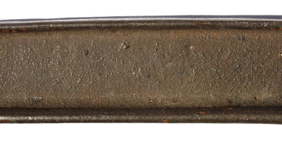
It’s worth showing a couple of images of mature rust surfaces in bright lighting to display the color (though model colors indoors should likely be darker). Here is a the body of a cast steel clamp:
And this next example shows how rust can develop and deepen when the steel is confined in a cavity (this is not typical of steel exposed in the open to moisture and lots of oxygen). In my view, few model railroad objects would need to be represented this way.

My usual approach to couplers in HO scale is to paint them with a flat, dirty black, with perhaps some dark brown on outer faces. Relatively few of my couplers have the entire body dark brown. I usually use Floquil “Roof Brown,” but a darker color would be as good or better. The goal is a pretty dark surface.
Here is just one example, in which the dark body of the coupler has been accented with brown. It is the chemical tank car described in a previous post (at: http://modelingthesp.blogspot.com/2012/10/small-modeling-project-icc-104-tank-car.html ). You can click to enlarge.

These examples show the way well-aged rust looks, and my primary example is the coupler surface. Other rust appearances will be the subject of a future post.
Tony Thompson
We all know that steel rusts when exposed to weather. And the sequence by which it happens is easy to observe for yourself. Put a piece of steel out in your yard, after cleaning with, say, steel wool, and observe what happens. If you live in a desert area, you may have to wait for rain, but in most of the U.S. moisture will arrive fairly quickly at this time of year. The first film on the steel will be a yellowish color, followed fairly soon by a reddish-orange that is a familiar rust color. But that changes to a solid brown color before long, and with further exposure, the brown gradually darkens.
So how do you show rust on your modeled objects? If it is something which has been exposed to weather only, and for some time, then it should be dark brown. Not light brown, not reddish-brown, but dark brown. If it is something which just had a paint failure, such as a scratch, you can show the pale yellow (indicating the rust just began within a couple of days) or red-orange for well-started rust, but remember that these indicate recent beginnings of rust.
There are two common railroad components which seem to be misunderstood by many modelers. First, couplers, the topic of this post. These are not supposed to be painted (though you will find exceptions), and they start rusting even before they are installed in a freight car. The great majority on almost any layout ought to be dark brown or darker. Why darker? Because dirt and oil get onto them also, and only the working faces, which get abraded, will be other than the very dark brown.
Let’s look at an example. This is a car about 15 years old, and probably it still has its original coupler. Here it is:
You can see what I described: a rather dark coupler body, with lighter brown rust on the working areas. And by the way, notice also the wheels, to which I will return in a moment: the wheel faces are entirely black.
Here is another coupler example, this a box car about five years old in an SP photo. It too has a rather dark coupler body with lighter working faces (click to enlarge):

My point is that couplers are dark and hardly noticeable as brown (except working faces). I will show a model example in a moment, but before I do, I should comment on my second topic, wheels. The same color appearance just described for couplers is also true of wheels on the inside of the wheelset, though the outside of wheelsets, the side we normally see, was so covered with accumulated journal oil plus dirt as to be entirely buried in blackish gunk. The flat car photo above shows this clearly. But you can do the dark brown rust on the inside surfaces of wheels if you like—it’s just pretty hard to see on other than tank cars.
It’s worth showing a couple of images of mature rust surfaces in bright lighting to display the color (though model colors indoors should likely be darker). Here is a the body of a cast steel clamp:

And this next example shows how rust can develop and deepen when the steel is confined in a cavity (this is not typical of steel exposed in the open to moisture and lots of oxygen). In my view, few model railroad objects would need to be represented this way.

My usual approach to couplers in HO scale is to paint them with a flat, dirty black, with perhaps some dark brown on outer faces. Relatively few of my couplers have the entire body dark brown. I usually use Floquil “Roof Brown,” but a darker color would be as good or better. The goal is a pretty dark surface.
Here is just one example, in which the dark body of the coupler has been accented with brown. It is the chemical tank car described in a previous post (at: http://modelingthesp.blogspot.com/2012/10/small-modeling-project-icc-104-tank-car.html ). You can click to enlarge.

These examples show the way well-aged rust looks, and my primary example is the coupler surface. Other rust appearances will be the subject of a future post.
Tony Thompson
Wednesday, December 5, 2012
Refrigerator car service terminology
I present talks about Pacific Fruit Express from time to time, and also touch on refrigerator car operations issues in some of my talks about waybills. In nearly every talk, there has been an audience question about the details of car operations and what is called “protective services,” meaning icing or other service to protect the load. This post is an attempt to clarify these services during the time of ice refrigeration. Much of what is in the post can also be found in the book, Pacific Fruit Express (A.W. Thompson, R.J. Church and B.H. Jones, 2nd edition, Signature Press, 2000). This book is still in print and available directly from the publisher, with free shipping.
Ice refrigerator cars had ice bunkers capable of holding around 10,000 pounds of ice, 5000 in each bunker. There were two ice hatches at each end of the car, but they opened into a single bunker at each end. Those familiar with today’s mechanical refrigeration may smile at 10,000 pounds of ice as a primitive measure, but in fact ice had a great advantage: the melting of ice consumes a great deal of heat. That in turn can rapidly cool the cargo in a car, or easily maintain a low temperature in the face of high external temperatures. It took some year before mechanical refrigeration equipment was developed with enough capacity to do the job which ice could do; the early mechanical reefers, in the period, say, from 1953 to 1960, were only suitable for loads which were already cold, such as frozen food, but did not have the capacity to cool a warm cargo sufficiently quickly.
The typical ice reefer was loaded at a shipper’s dock, then switched to an icing facility to fill the ice bunkers. Thereafter, it would be iced en route to market “as needed.” Often re-icing took place every 24 hours, but the interval could be specified by the shipper to be more often or less often, depending on estimates of en route outside temperatures. In re-icing, bunkers were simply refilled to the top, often taking several thousand pounds per bunker. At the ice deck, foremen with experience could estimate by eye the amount of ice which would be needed to fill the bunker, and the cost of that ice was charged to the shipper.
Here is a photo of a PFE workman at Ogden, Utah in 1962, carrying a clipboard on which to note the ice used. He is about to chalk a check mark on the inside of the hatch cover, to show that he has recorded the ice usage for this car, which had been chalked by a previous worker. This is a PFE photo from my collection.

Those icing costs, the official terminology of the services, and all details of providing services, along with the corresponding charges, were specified in the Perishable Protective Tariff, issued from time to time by the National Perishable Freight Committee in Chicago. For example, Tariff No. 11 was issued in 1940, Tariff No. 17 in 1957. These tariff had sections for each type of protective service. Most icing services were in Section 2; ventilation (open hatches) in Section 3; heater services to protect against cold in Section 4; and mechanical refrigeration in Section 5. This might be noted on a waybill as something like “CPS 3,” meaning “Carriers Protective Services, Section 3,” which would be ventilation. These tariffs are hundreds of pages long and contains remarkable levels of detail, far beyond what most modelers would need or want to know.
A much briefer and more convenient document, though still highly detailed, is the Code of Rules for Handling Perishable Freight, issued by the same committee, in the form of a series of circulars. Circular 20-A was issued in 1933 and by 1965 the series had reached Circular 20-F. These circulars of course use the same language as the tariffs. Let’s quickly summarize some of that language.
A shipper could order a car “pre-iced.” This means that the empty car had its ice bunkers filled before it was spotted at the shipper’s dock. This would help cool a hot car, in summer weather; and as the produce was loaded into the car, perhaps still warm from the field, there would be cold air inside, to start cooling the load toward its shipping temperature. But if the shipper was precooling his shipments in his own facility, there was much less need for pre-icing the car, and he would not want to pay for the pre-icing service. Note the terminology: that cars were pre-iced, loads were pre-cooled. This is the tariff language.
Once the car was loaded and picked up by a switch crew, it would be “initial iced,” meaning filling the bunker, whether or not it had been pre-iced. It would then head off toward market, being re-iced as needed in transit, perhaps several times if moving all the way across the country.
I have used these terminology details in my model waybills, as shown for example in this post: http://modelingthesp.blogspot.com/2011/08/waybills-10.html . I have varied the pre-icing and CPS sections appropriately for specific cargoes.
Modelers sometimes develop odd ideas about how ice was placed in bunkers. In actuality, it was done with three possible sizes of the ice (again, from tariff rules). These were as follows: “chunk,” meaning not more than 75 pounds per piece (a standard PFE ice block weighed 300 pounds, so that is a quarter of a block); “coarse,” meaning about the size of a melon, 10- to 20-pound pieces; and “crushed,” meaning about the size of a man’s fist. Any smaller than that, and there would not be large enough air spaces among the ice pieces to permit good air circulation, which of course was essential so that cold air from the bunker could move freely into the load space and displace warm air. But full 300-pound blocks were not placed directly in bunkers.
Other icing services included “top icing,” which involved blowing finely crushed ice across the top of the load inside the car, a good way to keep leafy vegetables moist in transit, and “body icing,” in which blocks of ice were placed among the boxes of produce. Some en-route icing stations could provide re-top-icing services.
These prototype details can be the basis for modeled operations and paperwork, such as waybills. Personally, I like to include what I can of prototype practices like these in the way I operate my layout.
Tony Thompson
Saturday, December 1, 2012
Vehicle license plates – trucks
In my original post on this topic, I primarily discussed automobile license plates, for my modeling locale of California in 1953. (You can see it at: http://modelingthesp.blogspot.com/2012/11/vehicle-license-plates-in-ho-scale.html ) Highway trucks were then, as now, issued license plates of a different format, and I wanted to model those properly also.
One of the kinds of model trucks I model is Pacific Motor Trucking or PMT, the SP’s intrastate motor trucking subsidiary. (It operated within all the states of SP’s Pacific Lines, but did not have interstate trucking authority, so highway operations could not cross state lines.) Here is a Southern Pacific photo of a new 1957 Ford cab-over, and this is typical of PMT license plates in the 1950s.

The license plate has an alphabetic character followed by five numbers. Here is a close-up view of it.

This type of plate is readily created by the same methods I described in my prior post on license plates, so that I can make plates like this:

This plate has a 1953 metal corner tag, as I described in my previous post.
I also mentioned commercial plates in my first post. Today, California classifies essentially any vehicle over 10,000 pounds gross weight as a commercial vehicle, and issues a corresponding plate. In the 1950s, in addition to the truck plates like Y93 218 above, commercial plates contained the word “COM,” as I showed in my previous post on license plates:

The California “COM” plate seems to have either been dropped altogether, or used only for a smaller class of vehicles, after the early 1950s. Accordingly, I am using it sparingly on my vehicles, in favor of the plate which has the format A00 000, shown above. These were also used for light trucks, such as pickups.
Here are some model examples. First, here is a PMT truck (custom decorated by Jim Elliot) on Chamisal Road alongside the Shumala depot, with its Y43 037 plate. You can click on the image to enlarge it.

Another example is this flatbed Chevrolet, with the Zaca Mesa winery behind it, at the Nipomo Street crossing in Ballard, with a “COM” plate, D72 019.

Finally, a pickup with a light truck plate, Y 930274, at the same location.

The point of this post is to illustrate that, as with automobiles, model trucks need license plates. Since many modelers tend to place a predominance of commercial buildings and industries on their layouts, it is natural that there are a corresponding lot of trucks, from pickups to semi-trailers, on those layouts, so the trucks are an important focus for model license plates.
Tony Thompson
Subscribe to:
Posts (Atom)